Introduction to the ‘baserater’ package
Introduction-to-the-baserater-package.RmdThe baserater package allows you to:
- Download a database of group–adjective pairs annotated with
stereotype strength scores generated by large language models (‘GPT-4’
and ‘LLaMA 3.3-70B’);
- Generate new typicality ratings using a large language model served
through any ‘Inference Provider’ API (e.g., ‘Together AI’ or
‘Fireworks’) of your choice, with customizable prompts and
parameters;
- Evaluate newly generated typicality ratings against human ground
truth (ratings collected from Prolific participants) and benchmark them
against baseline models;
- Automatically build a new base-rate item database from a group x description typicality matrix.
It is designed to streamline the creation of base-rate neglect items for reasoning experiments. A base-rate neglect item typically involves two groups (e.g., “engineers” and “construction workers”) and a descriptive trait (e.g., “nerdy”). Participants are presented with statistical information (base-rates; e.g., “There are 995 construction workers and 5 engineers”) and stereotypical information (the descriptive trait). Their task is to decide the most likely group membership of an individual described by that trait. The “typicality rating” generated by large language models quantifies how strongly certain traits (e.g., “nerdy,” “kind”) or descriptions are (stereo)typically associated with specific groups (e.g., engineers, nurses). This allows researchers to precisely measure and control “stereotype strength”–the extent to which a given description is perceived as belonging more strongly to one group over another (e.g., the trait “nerdy” is typically seen as more characteristic of engineers than of construction workers).
To learn more about the theoretical framework and validation studies
underlying the baserater package, see the paper: Using
Large Language Models to Estimate Belief Strength in Reasoning
(Beucler et al., 2025), available at https://doi.org/10.31234/osf.io/eqrfu_v1.
1. Downloading the Data
You can begin by downloading the article datasets using
download_data().
Use download_data() to retrieve either: - The full
base-rate item database (from ‘GPT-4’ and ‘LLaMA 3.3’); - The validation
ratings, which include human typicality scores and those generated by
‘GPT-4’ and ‘LLaMA 3.3’ on 100 group–adjective pairs. - The two
typicality matrices (from ‘GPT-4’ and ‘LLaMA 3.3’) that were used to
generate the base-rate item database. - The group and adjective material
used to build the database.
# Load the base-rate database
database <- download_data("database")

# Load the typicality validation ratings
ratings <- download_data("validation_ratings")

# Load the typicality matrices
gpt4_matrix <- download_data("typicality_matrix_gpt4")
llama3_3_matrix <- download_data("typicality_matrix_llama3.3")

# Load the group-adjective pairs
material <- download_data("material")
2. Generating New Typicality Ratings from LLMs
You can generate new typicality ratings using any ‘Inference
Provider’ API (e.g., ‘Together AI’, ‘Hugging Face’ Inference,
‘Fireworks’) via generate_typicality(). This feature is
experimental, as it depends on the provider’s API compatibility. See the
Inference Provider Setup section
at the end of this vignette for details on how to configure your API
endpoint and authentication token.
The function works by sending structured prompts to a large language model and parsing numeric outputs (between 0 and 100) that reflect how well a description (e.g., an adjective) fits a given group. By default, the function uses the same prompt and generation parameters described in the paper.
As in the paper, we output several ratings from the same model and average them to obtain a final score. The function allows you to specify the (minimum) number of responses to generate.
Note that the function generate_typicality() can be
quite slow, especially if you are generating many scores.
Here is an example of function call:
# Original prompt from the paper
original_system_prompt_content <- "You are expert at accurately reproducing the stereotypical associations humans make, in order to annotate data for experiments. Your focus is to capture common societal perceptions and stereotypes, rather than factual attributes of the groups, even when they are negative or unfounded."

original_user_prompt_content_template <- "Rate how well the adjective '{description}' reflects the prototypical member of the group '{group}' on a scale from 0 ('Not at all') to 100 ('Extremely').

To clarify, consider the following examples:

1. 'Rate how well the adjective FUNNY reflects the prototypical member of the group CLOWN on a scale from 0 (Not at all) to 100 (Extremely).' A high rating is expected because the adjective 'FUNNY' closely aligns with the typical characteristics of a 'CLOWN'.

2. 'Rate how well the adjective FEARFUL reflects the prototypical member of the group FIREFIGHTER on a scale from 0 (Not at all) to 100 (Extremely).' A low rating is expected because the adjective 'FEARFUL' diverges significantly from the typical characteristics of a 'FIREFIGHTER'.

3. 'Rate how well the adjective PATIENT reflects the prototypical member of the group ENGINEER on a scale from 0 (Not at all) to 100 (Extremely).' A mid-scale rating is expected because the adjective 'PATIENT' neither closely aligns nor diverges significantly from the typical characteristics of an 'ENGINEER'.

Your response should be a single score between 0 and 100, with no additional text, letters, or symbols included."


# Example using the validation ratings
groups <- ratings$group
descriptions <- ratings$adjective

api_token <- Sys.getenv("PROVIDER_API_TOKEN")

new_scores <- generate_typicality(
  groups                = groups,
  descriptions          = descriptions,
  api_url               = "https://api.together.xyz/v1/chat/completions", # example for 'Together AI' API
  api_token             =  api_token,
  model                 = "meta-llama/Meta-Llama-3.1-8B-Instruct-Turbo", #  model name on Together AI
  n                     = 3,  # number of responses to generate
  min_valid             = 2,  # minimum number of valid responses; mean of valid ones is used
  max_tokens            = 3,  # numeric output between 0 and 100
  retries               = 2,  # number of retries in case of API errors
  matrix                = FALSE,
  return_raw_scores     = TRUE,
  return_full_responses = TRUE,
  verbose               = TRUE)
Here is what the output looks like. Note that we could also see the
occasional error messages from the ‘Inference Provider’ API (e.g., too
many requests) since we set return_full_responses to
TRUE.
| group | description | mean_score | raw_scores | full_responses |
|---|---|---|---|---|
| DJ | naive | 22.33333 | 20, 12, 35 | 20, 12, 35 |
| accountant | solitary | 32.33333 | 42, 27, 28 | 42, 27, 28 |
| actor | altruistic | 23.66667 | 20, 30, 21 | 20, 30, 21 |
| aerobics instructor | impulsive | 60.33333 | 50, 38, 93 | 50, 38, 93 |
| architect | charismatic | 44.00000 | 55, 22, 55 | 55, 22, 55 |
| architect | reserved | 51.33333 | 60, 45, 49 | 60, 45, 49 |
We can also look at the distribution of the new typicality ratings generated by ‘LLaMA 3.1-8B-Instruct’:
# Distribution of new typicality ratings
ggplot(new_scores, aes(x = mean_score)) +
  geom_histogram(binwidth = 5, fill = "steelblue", color = "white") +
  labs(
    title = "Distribution of Typicality Ratings from 'LLaMA 3.1-8B-Instruct'",
    x = "Typicality Rating",
    y = "Count"
  ) +
  theme_classic()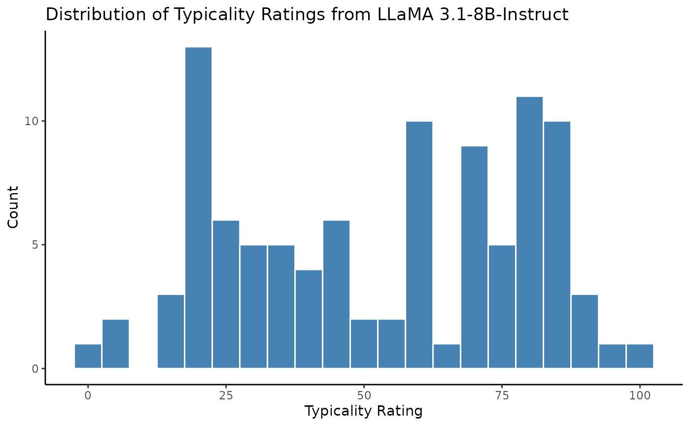
The generate_typicality() function supports two
modes:
-
matrix = TRUE(default): Computes a cross-product of unique groups and descriptions. Returns a list with matrices of scores and responses.
-
matrix = FALSE: Computes row-by-row scores for the group–adjective pairs you supply. Returns a tibble.
See ?generate_typicality for full documentation and
customization options.
3. Evaluating New Ratings
You can then assess how well a new model or scoring method captures group–adjective typicality by comparing your ratings to the human ground truth and benchmark models (‘GPT-4’ and ‘LLaMA 3.3’).
To do that, you need typicality ratings for the 100 validation items
stored in a data frame with three columns: group, adjective, and rating.
We will use the new_scores data frame we generated
earlier.
# Create a data frame with the same structure as the validation set
new_scores = new_scores %>%
  mutate(adjective = description,
         rating = mean_score) %>%
  select(group, adjective, rating)

knitr::kable(head(new_scores))| group | adjective | rating |
|---|---|---|
| DJ | naive | 22.33333 |
| accountant | solitary | 32.33333 |
| actor | altruistic | 23.66667 |
| aerobics instructor | impulsive | 60.33333 |
| architect | charismatic | 44.00000 |
| architect | reserved | 51.33333 |
First, let’s examine the correlation between the new scores and the human ratings visually:
# Join human and model scores
comparison_df <- left_join(
  ratings %>% select(group, adjective, human = mean_human_rating),
  new_scores,
  by = c("group", "adjective")
)

# Scatterplot
ggplot(comparison_df, aes(x = rating, y = human)) +
  geom_point(alpha = 0.6) +
  geom_smooth(method = "lm", se = FALSE, color = "darkred") +
  labs(
    title = "Scatterplot of 'LLaMA 3.1' and Human Typicality Ratings",
    y = "Average Human Rating",
    x = "Average 'LLaMA 3.1' Rating"
  ) +
  theme_classic()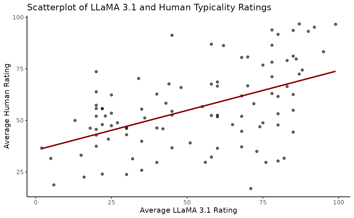
Use evaluate_external_ratings() to compute correlations
and display comparisons with our LLMs baseline:
# Print correlation summary with human ground truth and baselines
knitr::kable(evaluate_external_ratings(new_scores))| model | r | p |
|---|---|---|
| external | 0.6349740 | 0 |
| mean_gpt4_rating | 0.8848219 | 0 |
| mean_llama3_rating | 0.8179981 | 0 |
# Optionally store the output in a variable
results <- evaluate_external_ratings(new_scores)
As you can see, the smaller and older Llama-3.1-8B-Instruct does not perform as our baseline models (‘GPT-4’ and ‘LLaMA 3.3-70B’).
4. Constructing Base-Rate Items from Typicality Matrices
To compute stereotype strength using
extract_base_rate_items(), you’ll need a typicality
matrix—a table of scores where rows correspond to groups and columns
correspond to descriptions (e.g., adjectives). Each cell represents how
typical a description is for a group.
For example, you can load the ‘GPT-4’ typicality matrix using download_data() (the same is available for ‘LLaMA 3.3’):
#' The typicality matrix from 'GPT-4' is a data frame with group–adjective pairs and their typicality scores
gpt4_matrix <- download_data("typicality_matrix_gpt4")
knitr::kable(head(gpt4_matrix))| group | intelligent | arrogant | nerdy | kind | loud | careful | argumentative | persuasive | immature | active | funny | disorganized | dishonest | gentle | sensitive | creative | helpful | strong | brave | bossy | unconventional | quiet | organized | reliable | ambitious | charming | confident | efficient | friendly | generous | naive | witty | empathetic | stubborn | trustworthy | meticulous | inventive | charismatic | reserved | altruistic | original | impulsive | zealous | rational | idealistic | conservative | solitary | passionate | adventurous | cautious | extravagant | jovial | cooperative | attractive | muscular | shy | social | warm | moody | lazy | hardworking | imaginative | narrow-minded | boring | selfish | narcissistic |
|---|---|---|---|---|---|---|---|---|---|---|---|---|---|---|---|---|---|---|---|---|---|---|---|---|---|---|---|---|---|---|---|---|---|---|---|---|---|---|---|---|---|---|---|---|---|---|---|---|---|---|---|---|---|---|---|---|---|---|---|---|---|---|---|---|---|---|
| farmer | 55.00 | 15.20 | 11.6 | 75.32 | 13.8 | 84.04 | 21.20 | 25.6 | 12.60 | 88.20 | 22.4 | 20.6 | 14.20 | 63.08 | 34.80 | 38.80 | 80.00 | 88.0 | 70.60 | 19.80 | 20.8 | 71.40 | 83.8 | 85.44 | 50.40 | 33.6 | 74.60 | 79.32 | 79.60 | 65.6 | 28.80 | 29.6 | 48.80 | 71.80 | 84.4 | 71.00 | 53.40 | 28.4 | 67.8 | 62.60 | 37.2 | 19.60 | 51.6 | 76.80 | 34.60 | 80.60 | 74.80 | 75.2 | 31.60 | 77.80 | 10.0 | 61.40 | 79.4 | 31.00 | 78.0 | 26.40 | 33.20 | 70.40 | 22.20 | 10.20 | 91.00 | 32.6 | 36.24 | 38.00 | 17.80 | 10.20 |
| computer programmer | 90.28 | 57.80 | 85.2 | 42.20 | 13.4 | 84.40 | 30.20 | 33.4 | 32.96 | 28.40 | 25.0 | 35.0 | 19.20 | 37.08 | 33.00 | 74.00 | 54.80 | 25.8 | 22.60 | 21.40 | 71.2 | 76.20 | 82.2 | 83.00 | 81.00 | 26.4 | 69.20 | 86.16 | 42.28 | 35.4 | 19.60 | 42.8 | 33.20 | 66.00 | 70.2 | 84.60 | 85.92 | 26.6 | 79.2 | 30.80 | 72.6 | 20.60 | 73.4 | 86.52 | 33.00 | 36.20 | 80.00 | 75.6 | 26.20 | 76.60 | 15.6 | 22.20 | 51.8 | 28.40 | 14.8 | 74.68 | 32.00 | 24.32 | 43.20 | 26.80 | 85.00 | 70.4 | 29.40 | 66.40 | 25.20 | 24.60 |
| flight attendant | 50.20 | 27.68 | 11.4 | 84.00 | 21.2 | 83.92 | 20.72 | 39.0 | 15.60 | 84.44 | 30.8 | 16.6 | 15.40 | 77.00 | 73.32 | 30.80 | 86.88 | 34.4 | 40.72 | 36.60 | 26.0 | 31.00 | 87.8 | 82.80 | 36.20 | 75.0 | 82.80 | 82.40 | 85.40 | 48.2 | 17.72 | 49.0 | 77.20 | 20.60 | 81.8 | 80.40 | 24.00 | 73.4 | 30.4 | 59.04 | 24.2 | 21.32 | 56.6 | 69.40 | 21.20 | 29.80 | 14.00 | 58.2 | 70.28 | 73.96 | 19.0 | 74.08 | 86.0 | 79.60 | 18.4 | 18.20 | 85.60 | 78.20 | 30.40 | 15.00 | 86.60 | 26.4 | 16.00 | 19.72 | 18.08 | 21.60 |
| high school coach | 63.60 | 64.20 | 14.4 | 64.40 | 75.2 | 74.68 | 64.20 | 83.4 | 20.52 | 88.40 | 40.8 | 29.8 | 27.16 | 36.40 | 35.32 | 56.40 | 85.20 | 86.0 | 71.00 | 79.68 | 26.8 | 23.52 | 79.0 | 78.60 | 79.44 | 39.8 | 85.08 | 69.80 | 74.44 | 64.8 | 19.60 | 42.2 | 65.20 | 72.60 | 75.2 | 61.80 | 49.40 | 76.0 | 29.6 | 70.08 | 38.4 | 36.40 | 81.6 | 73.40 | 54.24 | 69.00 | 20.00 | 86.6 | 61.60 | 70.80 | 16.8 | 71.00 | 79.8 | 40.72 | 81.4 | 17.00 | 77.52 | 64.48 | 32.72 | 25.20 | 84.80 | 41.4 | 48.48 | 34.28 | 28.84 | 32.48 |
| dentist | 85.92 | 39.88 | 23.8 | 60.80 | 10.4 | 90.60 | 18.80 | 53.6 | 11.08 | 37.80 | 20.0 | 15.4 | 22.52 | 75.40 | 39.80 | 35.12 | 81.40 | 29.6 | 30.60 | 30.40 | 19.2 | 70.20 | 88.0 | 85.60 | 69.80 | 33.2 | 84.80 | 83.40 | 69.40 | 35.6 | 11.60 | 26.2 | 53.88 | 26.64 | 81.6 | 89.60 | 31.00 | 35.0 | 63.6 | 36.00 | 27.6 | 18.00 | 37.2 | 85.00 | 19.20 | 52.40 | 35.52 | 55.8 | 21.80 | 86.20 | 27.0 | 26.00 | 72.8 | 37.60 | 18.2 | 20.80 | 36.80 | 33.40 | 20.48 | 14.28 | 86.32 | 29.4 | 17.76 | 65.08 | 26.68 | 20.80 |
| lawyer | 85.20 | 74.28 | 33.0 | 33.80 | 39.6 | 83.40 | 83.80 | 88.6 | 18.00 | 73.80 | 20.4 | 20.2 | 69.40 | 26.40 | 29.60 | 43.60 | 47.80 | 68.4 | 33.40 | 70.20 | 22.4 | 26.20 | 86.0 | 64.60 | 87.60 | 35.4 | 87.00 | 74.60 | 36.00 | 31.2 | 14.20 | 69.0 | 32.80 | 70.80 | 42.0 | 83.88 | 46.00 | 69.2 | 40.2 | 28.60 | 39.8 | 25.28 | 74.0 | 84.80 | 27.80 | 61.68 | 34.00 | 70.6 | 30.80 | 83.00 | 66.2 | 20.80 | 47.8 | 41.52 | 16.2 | 18.60 | 63.32 | 22.20 | 30.40 | 19.80 | 85.20 | 37.6 | 31.40 | 62.20 | 71.00 | 67.60 |
Extract base-rate items by applying the function:
#' Extract base-rate items from the typicality matrix
base_rate_items <- extract_base_rate_items(gpt4_matrix)
Note that the function extract_base_rate_items() can
take some time to run if you are using a large matrix, as this will
create a very large number of items (e.g., here, around 110,000
base-rate items).
You can then explore or filter the output, e.g., to view the strongest stereotypes:
# View top base-rate items by stereotype strength
knitr::kable(base_rate_items %>%
  arrange(desc(StereotypeStrength)) %>%
head(10))| Group1 | Group2 | Description | Score1 | Score2 | StereotypeStrength |
|---|---|---|---|---|---|
| fashion designer | paramedic | extravagant | 82.80 | 8.0 | 2.336987 |
| fashion model | paramedic | extravagant | 79.60 | 8.0 | 2.297573 |
| music producer | paramedic | extravagant | 78.04 | 8.0 | 2.277780 |
| hippy | fitness trainer | lazy | 72.00 | 7.4 | 2.275186 |
| drummer | librarian | loud | 83.60 | 8.6 | 2.274281 |
| politician | fitness trainer | lazy | 71.44 | 7.4 | 2.267378 |
| politician | paramedic | extravagant | 76.00 | 8.0 | 2.251292 |
| DJ | librarian | loud | 81.20 | 8.6 | 2.245153 |
| aerobics instructor | librarian | loud | 80.60 | 8.6 | 2.237736 |
| politician | paramedic | selfish | 83.64 | 9.0 | 2.229297 |
You can also subset the database to focus on a specific adjective or group. For example, you can visualize the stereotype strength of the adjective “selfish” across group combinations:
# Pick one adjective and extract group typicality scores
df <- gpt4_matrix %>%
  select(group, selfish) %>%
  rename(score = selfish) %>%
  arrange(desc(score))  # sort by how typical the group is

# Save group names and their scores
group_order <- df$group
typ_values  <- df$score
names(typ_values) <- df$group

# Build all group pairs and compute log-ratios
res_df <- expand.grid(
  g1 = group_order,
  g2 = group_order,
  KEEP.OUT.ATTRS = FALSE
) %>%
  mutate(
    typ1 = typ_values[as.character(g1)],
    typ2 = typ_values[as.character(g2)],
    log_ratio = log(pmax(typ1, 1e-9) / pmax(typ2, 1e-9))
  ) %>%
  mutate(
    g1 = factor(g1, levels = group_order),
    g2 = factor(g2, levels = group_order)
  )

# Keep only pairs where g1 is ranked higher than g2 and log-ratio is positive
res_df <- res_df %>%
  filter(as.integer(g1) < as.integer(g2), log_ratio > 0)

# Add identity pairs (g1 == g2) with NA
diag_df <- tibble(
  g1 = factor(group_order, levels = group_order),
  g2 = factor(group_order, levels = group_order),
  log_ratio = NA_real_
)

# Combine with original filtered upper-triangle pairs
res_df <- bind_rows(res_df, diag_df)

# Plot the heatmap
ggplot(res_df, aes(x = g2, y = g1, fill = log_ratio)) +
  geom_tile(color = "white") +
  scale_fill_gradient2(
    low       = "steelblue",
    mid       = "white",
    high      = "firebrick",
    midpoint  = 0,
    na.value  = "grey90",
    name      = "Log(Group 1 / Group 2)",
  ) +
  labs(
    title = "Stereotype Strength for Adjective 'Selfish'",
    x = "Group 2",
    y = "Group 1"
  ) +
  theme_classic() +
  theme(
    axis.text.y = element_text(angle = 15, hjust = 1, size = 5),
    axis.text.x = element_text(angle = 45, hjust = 1, size = 5),
    panel.grid  = element_blank()
  )
Citation
If you use baserater in your research, please cite:
Beucler, J. (2025). baserater: An R package using large language models to estimate belief strength in reasoning. R package version 0.1.2. https://doi.org/10.32614/CRAN.package.baserater
Inference Provider Setup
The baserater package can connect to inference providers
such as ‘Together AI’, ‘Hugging Face’ Inference, ‘Fireworks’, and
‘Replicate’. These platforms host or serve large language models and
allow you to query them through a standard HTTP interface.
Here are some useful links to get started:
To generate new scores using the generate_typicality()
function, complete the following setup steps:
Obtain your provider’s API URL and token:
Optionally, store them as environment variables in R, for example:Sys.setenv(PROVIDER_API_URL = "https://api.together.xyz/v1/chat/completions")Sys.setenv(PROVIDER_API_TOKEN = "your_secret_token")Check model availability and license terms:
Some models require that you agree to license terms before use. Check the provider’s model catalog for details.Verify the correct model identifier for your provider:
Model names can vary depending on the provider (for example,"meta-llama/Llama-3.3-70B-Instruct-Turbo"on ‘Together AI’ vs."meta-llama/Llama-3.3-70B-Instruct"on ‘Hugging Face’). Always use the exact identifier listed in the provider’s documentation.